Prokaryote Standard
Project Description
Objective: Generate an metagenomics summary report, with the goal of reconstructing and characterizing prokaryotic genomes.
Full data is available at /fs/ess/PAS2095/CoMS/test_dataset/prokaryote_std/. There are 10 samples. The average read depth is 104M reads with a range from 38M to 142M reads and a standard deviation of 36M reads.
Workflow overview: Illumina sequencing reads were first checked for quality and used to generate separate assemblies for each sample. From each assembly, we then sorted contigs into genome bins, which were assessed for quality based on genome completion and contamination. Medium and high-quality bins (>=70% completion, <10% contamination; >=95% completion <5% contamination respectively) were retained as metagenome assembled genomes (MAGs). We then taxonomically classified and generated a metabolism/functional profile for each MAG. Community composition across samples was then assessed by two approaches, first based on read coverage on a set of reference single copy marker genes, and second, based on read coverage of the high and medium quality MAGs.
There is much more valuable data than what can be reasonably presented in this report at the directory noted above. I suggest that we meet to discuss these results in detail at your earliest convenience.
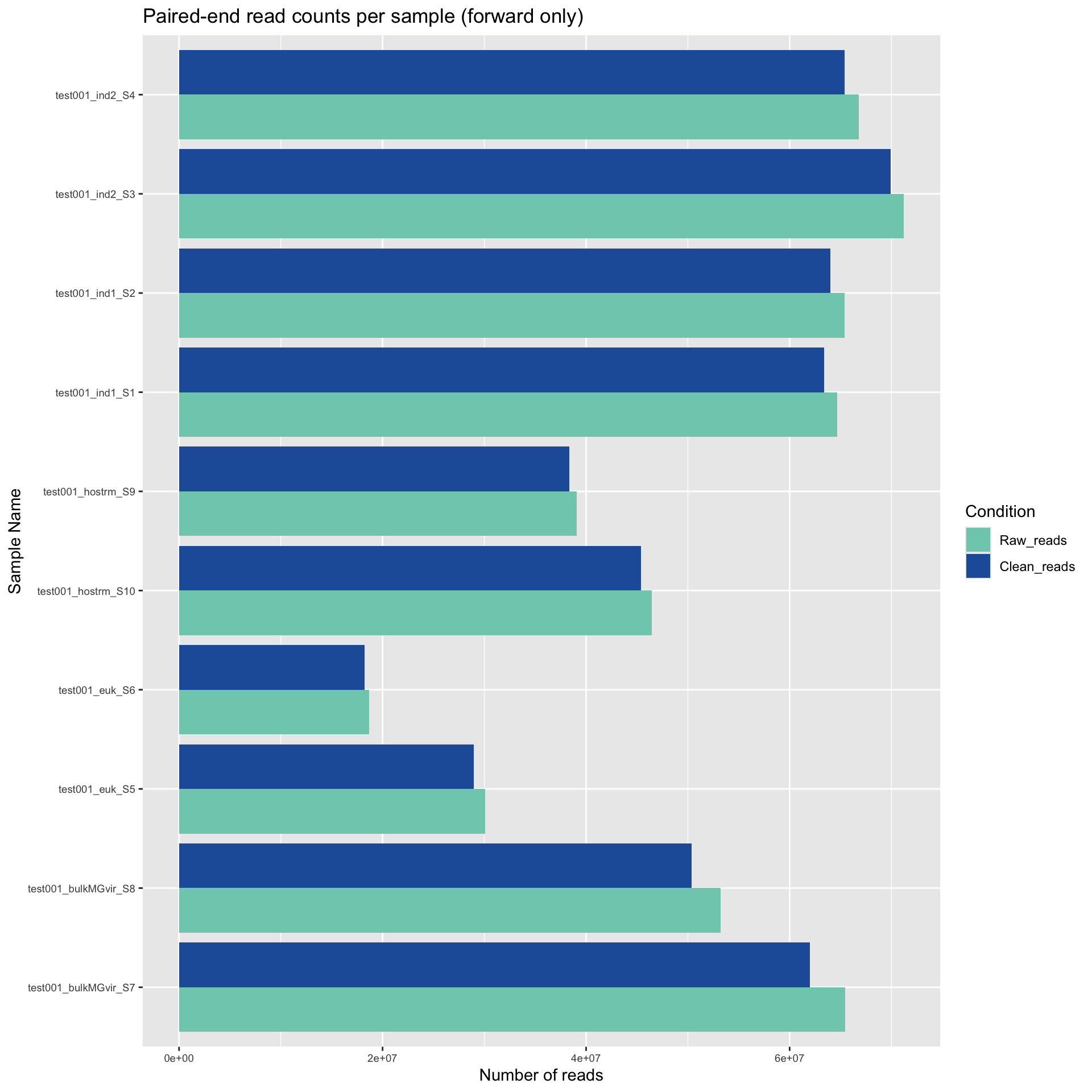
For each sample, we filtered the “raw reads” produced from Illumina sequencing for quality and adapter sequences. Here, we used Trimmomatic (Bolger et al., 2014) to remove bases with low quality and any remaining sequencing adapters. This filtering results in “cleaned reads”. The cleaned reads are then used for further analysis.
Here, we plotted the number of raw reads and cleaned reads for each sample. Note that these are paired read counts. For “sequencing depth”, multiply these values by 2.
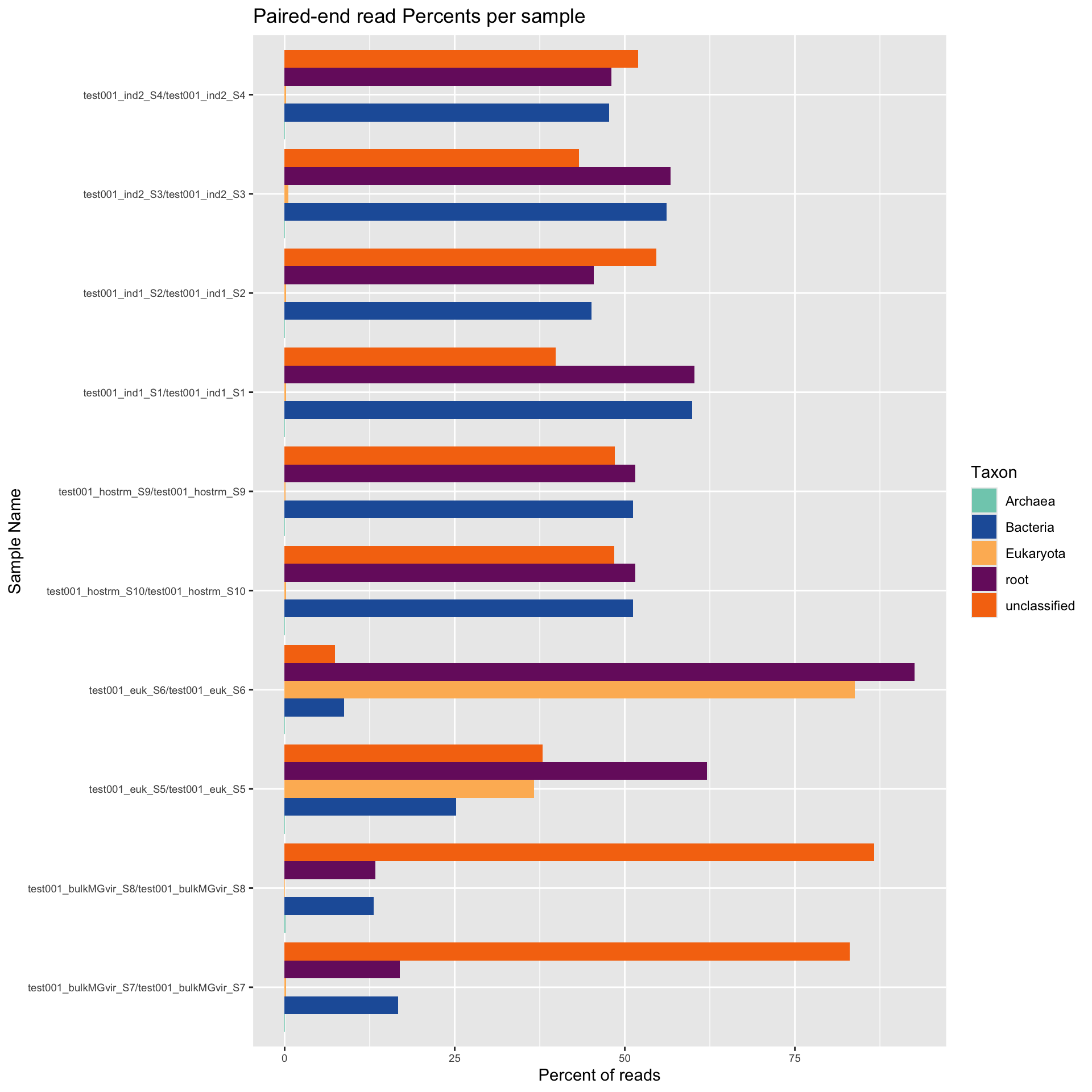
Using Kraken2 Kraken2 (Wood et al., 2019) we next assess the proportion of reads assigned to Eukaryota, Bacteria, or Archaea. In this instance, the category “Root” is the proportion of total reads that obtain any classification at all. The following categories “Eukaryota”, “Bacteria”, “Archaea” or “Unclassified” represent the breakdown of “Root” into each respective domain.
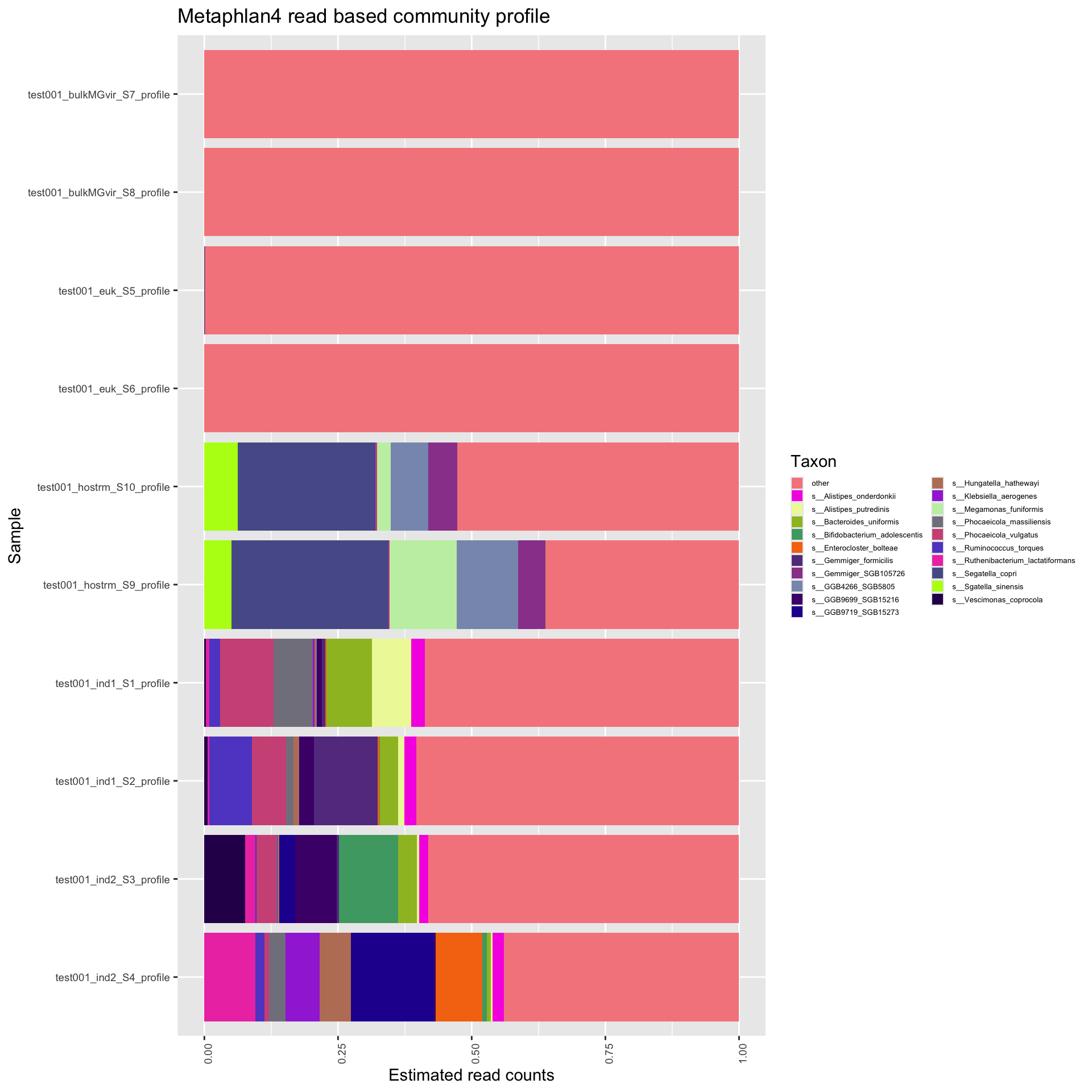
To generate a preliminary community profile, we use Metaphlan4 with the database mpa_vJun23_CHOCOPhlAnSGB_202403 (Blanco-Miguezet al.,) with the option -t rel_ab_w_read_stats to estimate read counts (required for certain downstream analysis). These community profiles per sample were then merged and simplified to represent only the species-level counts. Below we plot only the 20 most prevalent species across all samples, with all other species collapsed to “other”. Please note that read-based community profilers are only as accurate as their database is representative of a given sample and often substantially overestimate alpha diversity. These data should be inspected critically.
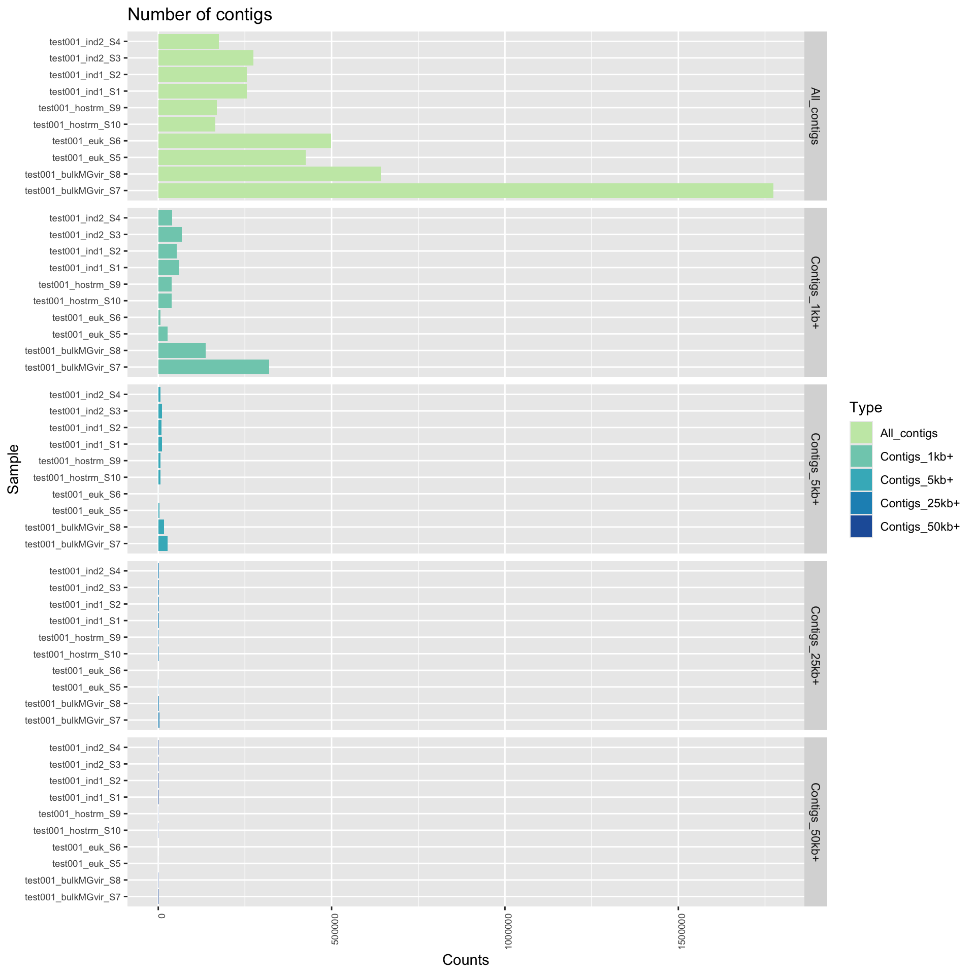
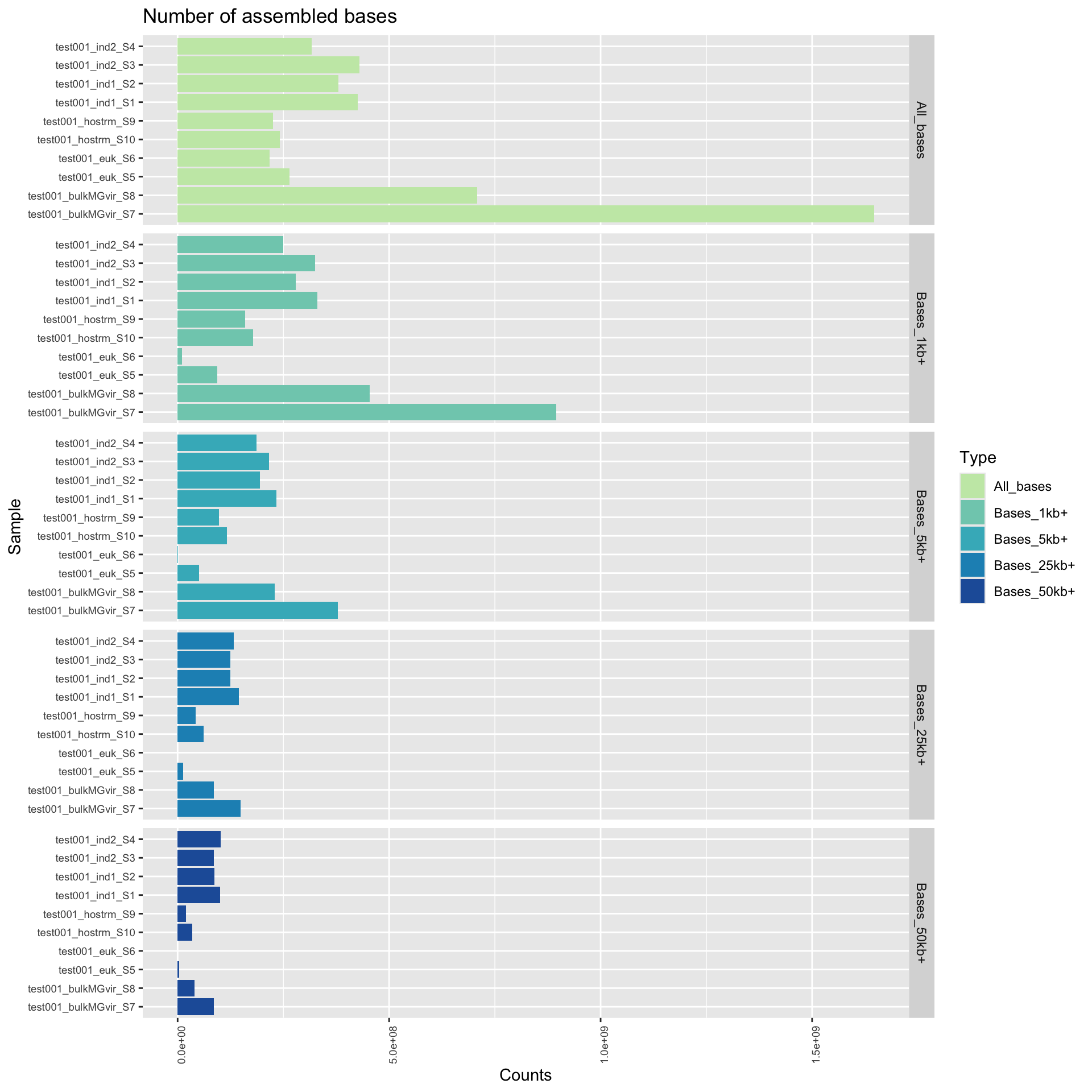
For each sample, genomes were assembled into contigs with MEGAHIT (Li et al., 2015). Genome assembly metrics were assessed with QUAST (Gurevich et al., 2013). Some important factors include the number of contigs, and the number of bases assembled, measured using different sequence length cut-offs in each individual sample. Some other common statistics (like N50) are included in the data files.
Here, we plot both the number of contigs, categorized by contig length. These graphs provide an overview of how fragmentation of each assembly and how the assembled bases are distributed. This will be impacted by sequencing depth as well as community complexity so it is important to put these result in context. If there are issues with identifying a comprehensive set of genome bins, we would examine these assembly statistics to assess due to fragmentation. For example, it is common to have many small fragments (under 1,000 bp). However, if a disproportionately large amount of bases are distributed to small fragments, that is indicative of a relatively poor assembly.
We used part of the MetaWRAP (Uritsky et al., 2018) pipeline to “bin” assembled contigs into genomes and assess quality. This pipeline uses MetaBat2 (Kang et al., 2019), MaxBin2 (Simmons et al., 2016), and CONCOCT (Lu et al., 2017) for binning and chooses the best version of each genome bin across the binning tools. These genome bins were de-replicated at 98% average nucleotide identity (ANI) across samples with dRep (Olm et al., 2017). These genome bins are generally referred to as metagenome-assembled genomes (MAGs) from this point on.
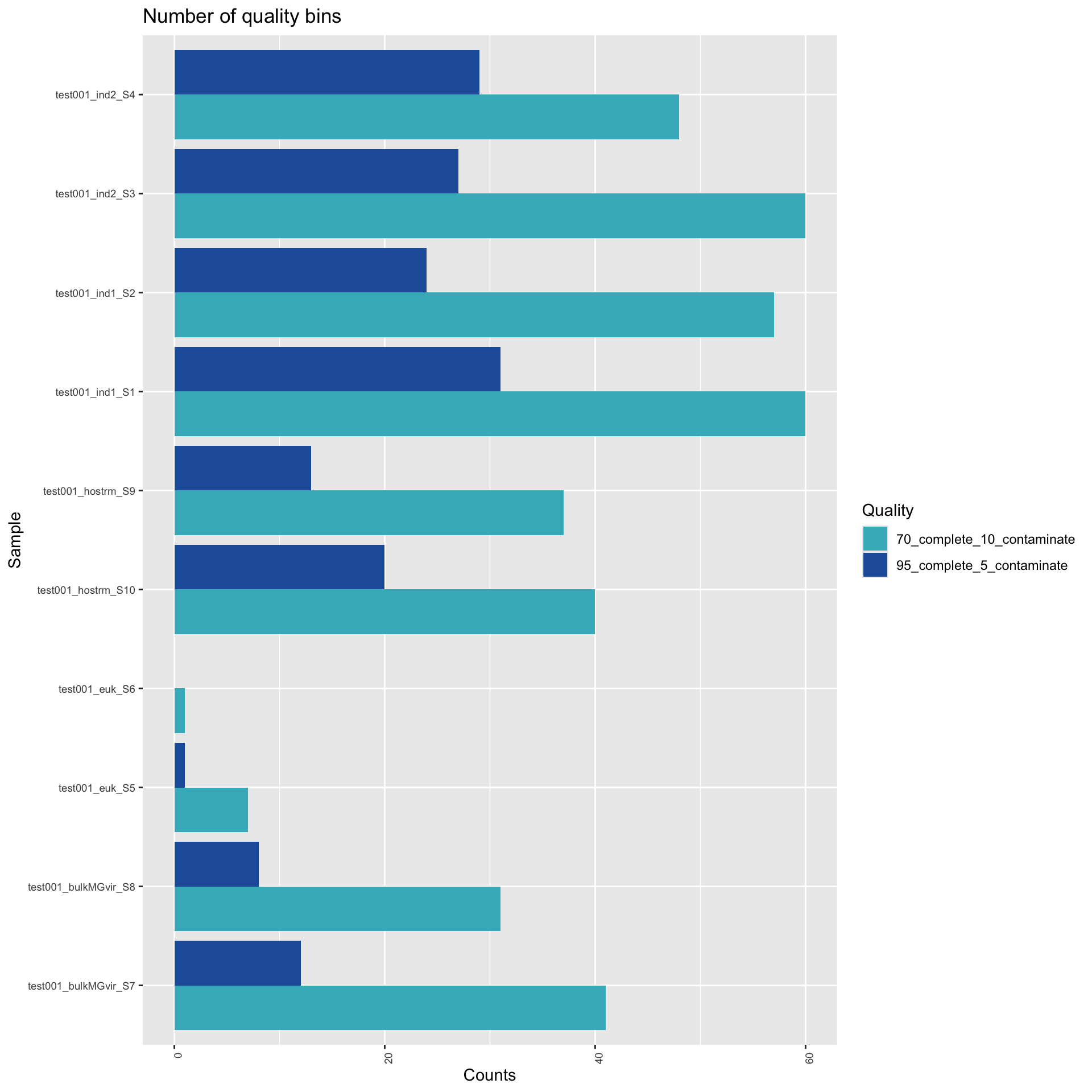
The field standard is to evaluate these MAGs for genome completeness and contamination with CheckM (Parks et al., 2015). From Parks et al, 2015: “Genome completeness is estimated as the number of marker sets present in a genome taking into account that only a portion of a marker set may be identified”; “Genome contamination is estimated from the number of multi-copy marker genes identified in each marker set.” Only MAGs with >70% completion and <10% contamination (medium quality) are considered, with high quality denoting MAGs with >95% completion and <5% contamination.
Taxonomy for each MAG was assigned with GTDBTk (Chaumeil et al., 2020), which assigns “objective taxonomic classifications to bacterial and archaeal genomes based on the Genome Database Taxonomy (GTDB).”
Here, we show the number of dereplicated MAGs by quality, in the plot below. Further, the table below shows a (searchable/sortable) summary table of all MAGs detected, along with the taxonomic classification, completeness, contamination, and quality.
Show 102550100 entries
| Bin | Taxonomic_classification | completeness | contamination |
|---|---|---|---|
| test001_bulkMGvir_S7metawrap_70_10_bins_bin.10 | g__Bog-1198 | 90.94 | 5.721 |
| test001_bulkMGvir_S7metawrap_70_10_bins_bin.11 | g__RAAP-2 | 92.3 | 1.282 |
| test001_bulkMGvir_S7metawrap_70_10_bins_bin.12 | g__Palsa-1447 | 98.63 | 3.082 |
| test001_bulkMGvir_S7metawrap_70_10_bins_bin.13 | f__Polyangiaceae | 83.83 | 3.569 |
| test001_bulkMGvir_S7metawrap_70_10_bins_bin.14 | g__Palsa-744 | 88.05 | 1.082 |
| test001_bulkMGvir_S7metawrap_70_10_bins_bin.15 | s__RAAP-2 | 88.81 | 1.709 |
| test001_bulkMGvir_S7metawrap_70_10_bins_bin.16 | g__UBA11358 | 93.91 | 6.612 |
| test001_bulkMGvir_S7metawrap_70_10_bins_bin.17 | g__FEN-1191 | 82.03 | 5.488 |
| test001_bulkMGvir_S7metawrap_70_10_bins_bin.18 | f__Obscuribacteraceae | 95.72 | 1.851 |
| test001_bulkMGvir_S7metawrap_70_10_bins_bin.19 | s__RAAP-2 | 96.33 | 4.31 |
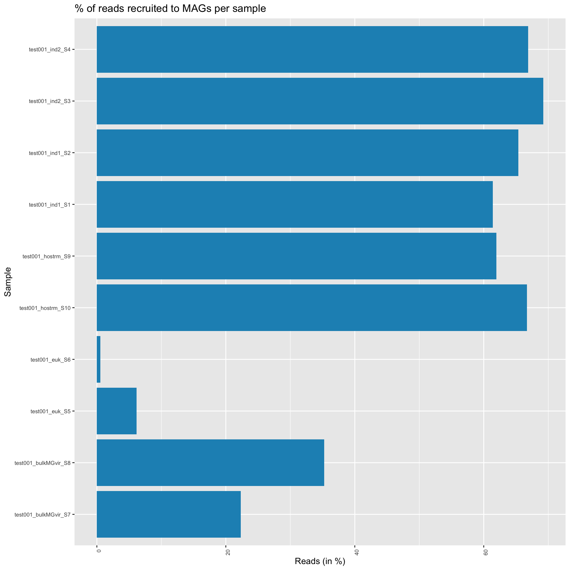
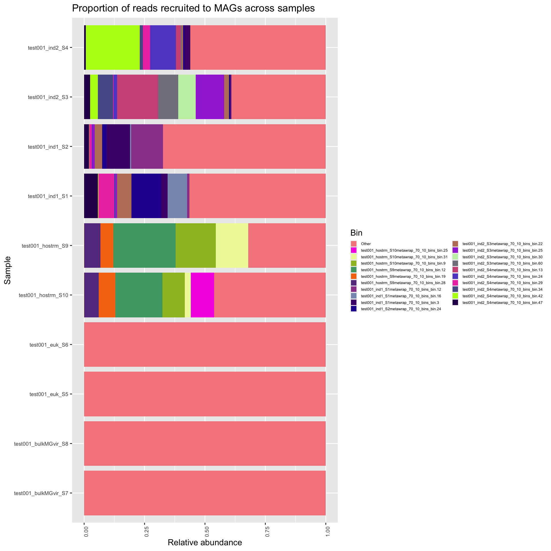
Community profiles can also be generated by tracking MAGs (which have a taxonomic classification) and their abundance (via read recruitment) across all samples within the project. We used CoverM to generate an abundance table of trimmed mean read coverage (the average coverage after removing the 5% of bases with highest and lowest coverage). Coverages normalized by sequencing depth are provided in the data files and represent a proxy for MAG relative abundance, which can be used for most downstream community ecology analysis.
Here, we first plot the proportion of reads that map to the MAGs. This gives us a estimation of how representative the MAGs are of the sample. For downstream ecological analysis, we want this number to be relatively high (arbitrarily). The second plot shows the MAG abundances per sample, including only the quality dereplicated MAGs from above, and presenting only the 20 most prevalent bins across all samples, with the rest collapsed to “other”. The relative abundances are taken from all reads recruited and does not take into reads that failed to recruit.
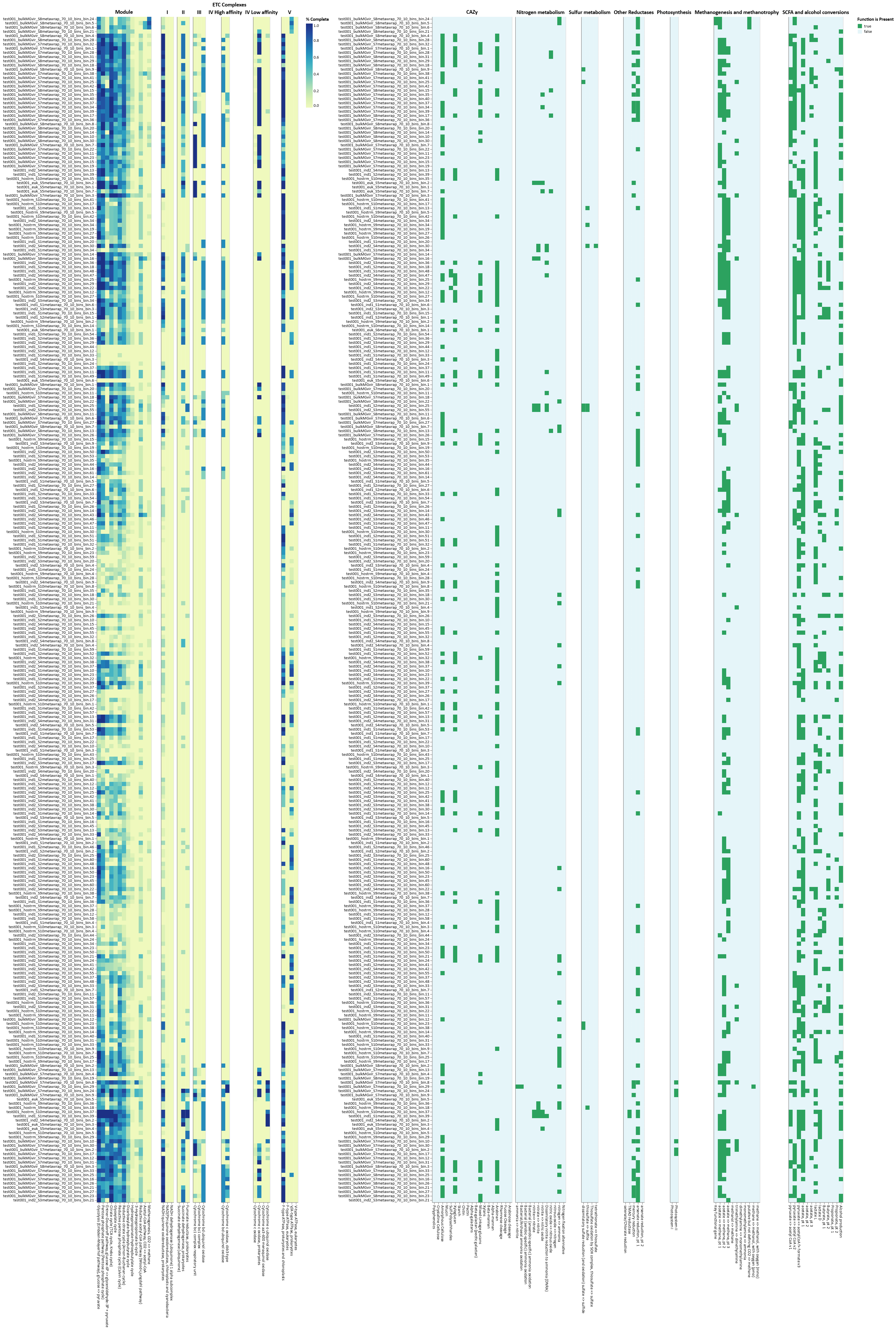
Functional annotations are provided per dereplicated MAG with DRAM version 1.3 Shaffer et al., 2020 using the option ”annotate” and the non-licensed version of KEGG (Kanehisa et al., 2000) KO-fam. These annotations are further summarized with DRAM’s “distill” function (Shaffer et al., 2020), providing per genome/ per sample/ or per treatment (if provided) metabolic information.
Here we displayed the summary metabolic information for “Core metabolism” and “Assimilatory and Dissimilatory functions” per sample as the proportion of MAGs in a given sample with a complete metabolic category (completeness calculated by DRAM - see link above), and “Assimilatory and Dissimilatory functions” per genome as the presence/absence for each metabolic category in each genome bin, broken into sample level groups. Full functional annotations per genome, per gene, and much more detailed summary metabolic information are provided in the data files.